Conditional Formatting
Conditional formatting allows you to apply various formatting styles (color, font, decoration, gradient) to cells to work with data on the spreadsheet: highlight or sort through and display the data that meets the needed criteria. Specify the fit for purpose criteria and create new formatting rules, edit, manage or clear the existing rules.
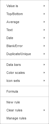
Conditional formatting rules supported by the ONLYOFFICE Spreadsheet Editor are:
Value is, Top/Bottom, Average, Text, Date, Blank/Error, Duplicate/Unique, Data Bars, Color Scales, Icon Sets, Formula.
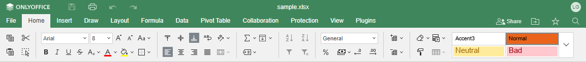
For quick access, or if you want to choose one of the available preset conditions, or to access all the available conditional formatting options go to the Home tab and click the Conditional formatting button .
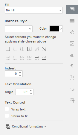
All Conditional Formatting options are also available on the right sidebar in the Cell Settings tab. Click the Conditional Formatting control down arrow to open the drop-down menu containing all the available options.
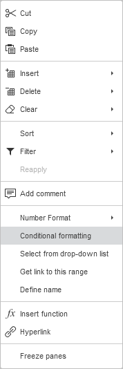
To open the New Formatting Rule window, you can right-click any cell and choose Conditional Formatting from the contextual menu.
To apply a formatting rule condition, select the cell range then click the Conditional formatting button on the top toolbar, or click the Conditional Formatting control of the Cell Settings tab on the right sidebar, and choose the appropriate rule from the drop-down menu.
 .
.
The New Formatting Rule window will open for you to format the highlighting criteria.
Value is Formatting Rule
The Value is formatting rule is used to find and highlight cells meeting a certain comparison condition:
- Greater than
- Greater than or equal to
- Less than
- Less than or equal to
- Equal to
- Not equal to
- Between
- Not between

- The Rule section shows the selected rule and the selected comparison condition, by clicking the down arrow you can access the list of the available rules and conditions. Use the Select Data box to define the cell value to compare with. Use the reference to a single cell, or the reference with the worksheet function such as =SUM(A1:B5).
- The Format section offers a range of cell formatting options. You can choose one of the available format Presets
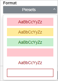
or
customize the formatting using font format options (Bold, Italic, Underline, Strikeout), Text color, Fill color and Borders. Use the General drop-down list to choose the appropriate number format (General, Number, Scientific, Accounting, Currency, Date, Time, Percentage). The Preview box shows how the cell will look like after formatting. Click the Clear
to delete all the formatting.
Click OK to confirm.
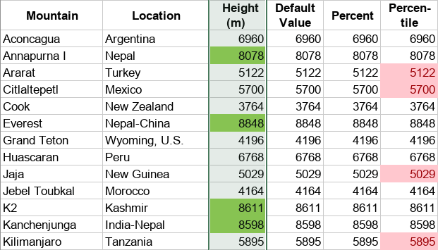
The example below illustrates the preset formatting criteria, such as Greater than, and Between. This formats mountains with a height greater than 6,960 with a green background and percentile between 5,000 and 6,500 with pink.
Top/Bottom Formatting Rule
The Top/Bottom rule is used to find and display the top and bottom values within the spreadsheet:
- Top 10 items
- Top 10%
- Bottom 10 items
- Bottom 10%
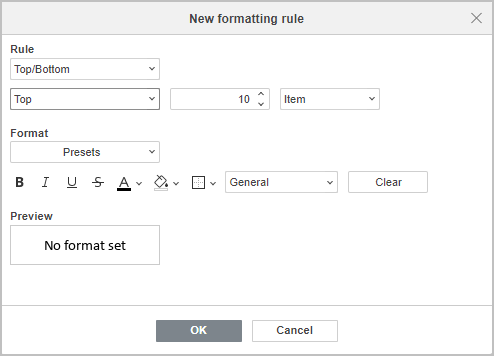
- The Rule section shows the selected rule and the selected condition, by clicking the down arrow you can access the list of the available rules and conditions, the number of items (percentage) to display, and choose either you want to highlight items or percentage.
- The Format section offers a range of cell formatting options. You can choose one of the available format Presets
or
customize the formatting using font format options (Bold, Italic, Underline, Strikeout), Text color, Fill color and Borders. Use the General drop-down list to choose the appropriate number format (General, Number, Scientific, Accounting, Currency, Date, Time, Percentage). The Preview box shows how the cell will look like after formatting. Click the Clear button to delete all the formatting.
Click OK to confirm.
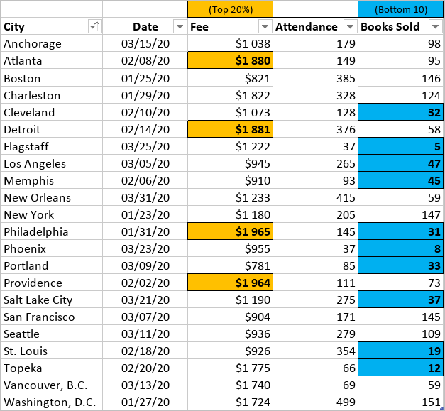
The example below illustrates the preset formatting criteria, such as Top 10% set to show top 20% values, and Bottom 10 items. This formats Top 20% of fees in the cities you visited with an orange background and bottom values for cities where you sold a small number of books with a blue background.
Average Formatting Rule
The Average is used to find and display values above or below an average or standard deviation in a rating:
- Above
- Below
- Equal to or above
- Equal to or below
- 1 std dev above
- 1 std dev below
- 2 std dev above
- 2 std dev below
- 3 std dev above
- 3 std dev below
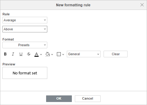
- The Rule section shows the selected rule and the selected condition, by clicking the down arrow you can access the list of the available rules and conditions.
- The Format section offers a range of cell formatting options. You can choose one of the available format Presets
or
customize the formatting using font format options (Bold, Italic, Underline, Strikeout), Text color, Fill color and Borders. Use the General drop-down list to choose the appropriate number format (General, Number, Scientific, Accounting, Currency, Date, Time, Percentage). The Preview box shows how the cell will look like after formatting. Click the Clear button to delete all the formatting.
Click OK to confirm.
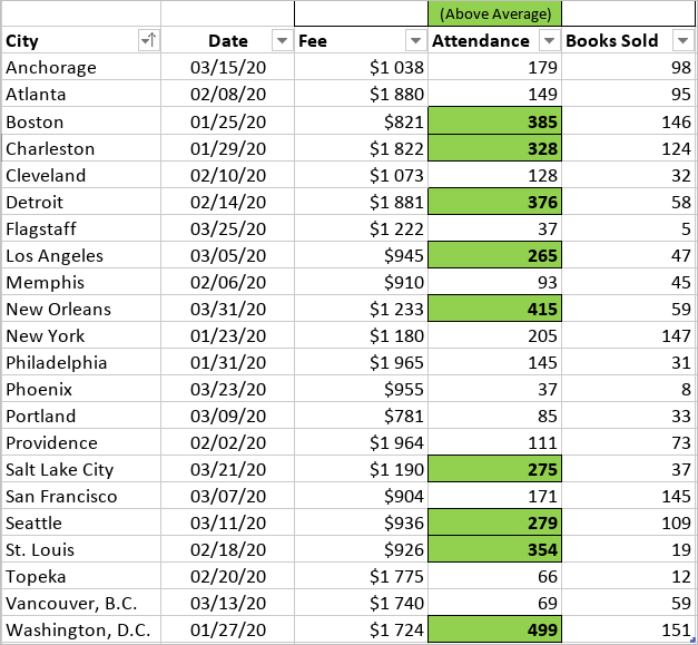
The example below illustrates the preset formatting criteria, such as Above average. This formats the cities where the attendance was above average with a green background.
Text Formatting Rule
The Text formatting rule is used to find and highlight cells containing certain text and meeting one of the available formatting conditions:
- Contains
- Does not contain
- Begins with
- Ends with

- The Rule section shows the selected rule and the selected formatting condition, by clicking the down arrow you can access the list of the available rules and conditions. Use the Select Data box to define the cell value to compare with. Use the reference to a single cell, or the reference with the worksheet function such as =SUM(A1:B5).
- The Format section offers a range of cell formatting options. You can choose one of the available format Presets
or
customize the formatting using font format options (Bold, Italic, Underline, Strikeout), Text color, Fill color and Borders. Use the General drop-down list to choose the appropriate number format (General, Number, Scientific, Accounting, Currency, Date, Time, Percentage). The Preview box shows how the cell will look like after formatting. Click the Clear button to delete all the formatting.
Click OK to confirm.
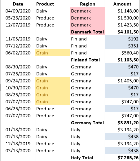
The example below illustrates the preset formatting criteria, such as Contains. This formats cells containing Denmark with a pink background to highlight sales for a specific region.
Date Formatting Rule
The Date formatting rule is used to find and highlight cells containing a certain date and meeting one of the available formatting conditions:
- Yesterday
- Today
- Tomorrow
- In the last 7 days
- Last week
- This week
- Next week
- Last month
- This month
- Next month
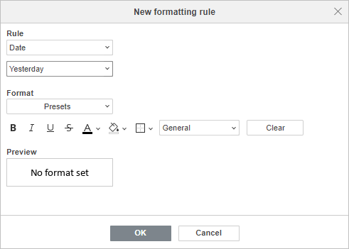
- The Rule section shows the selected rule and the selected formatting condition, by clicking the down arrow you can access the list of the available rules and conditions.
- The Format section offers a range of cell formatting options. You can choose one of the available format Presets
or
customize the formatting using font format options (Bold, Italic, Underline, Strikeout), Text color, Fill color and Borders. Use the General drop-down list to choose the appropriate number format (General, Number, Scientific, Accounting, Currency, Date, Time, Percentage). The Preview box shows how the cell will look like after formatting. Click the Clear button to delete all the formatting.
Click OK to confirm.
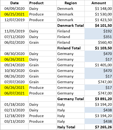
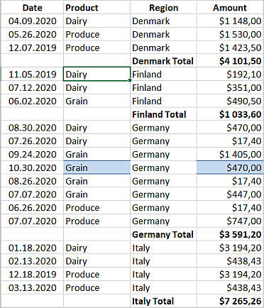
The example below illustrates the preset formatting criteria, such as Last month. This formats cells containing dates from the previous month with a yellow background to highlight sales for a specific period of time.
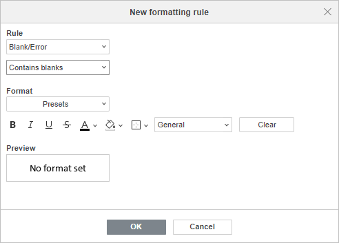
Blank/Error Formatting Rule
The Blank/Error formatting rule is used to find and highlight cells containing or not containing blanks and errors:
- Contains blanks
- Does not contain blanks
- Contains errors
- Does not contain errors
- The Rule section shows the selected rule and the selected formatting condition, by clicking the down arrow you can access the list of the available rules and conditions.
- The Format section offers a range of cell formatting options. You can choose one of the available format Presets
or
customize the formatting using font format options (Bold, Italic, Underline, Strikeout), Text color, Fill color and Borders. Use the General drop-down list to choose the appropriate number format (General, Number, Scientific, Accounting, Currency, Date, Time, Percentage). The Preview box shows how the cell will look like after formatting. Click the Clear button to delete all the formatting.
Click OK to confirm.
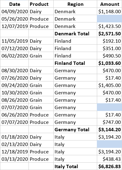
The example below illustrates the preset formatting criteria, such as Contains blanks. This formats blank cells in the column showing the number of sales with a light blue background.
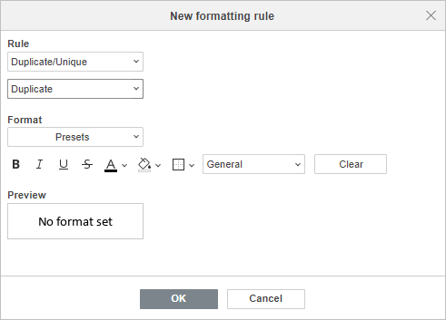
Duplicate/Unique Formatting Rule
The Duplicate/Unique formatting rule is used to display duplicate values within the spreadsheet and the cell range defined by the conditional formatting, the available options are:
- The Rule section shows the selected rule and the selected formatting condition, by clicking the down arrow you can access the list of the available rules and conditions.
- The Format section offers a range of cell formatting options. You can choose one of the available format Presets
or
customize the formatting using font format options (Bold, Italic, Underline, Strikeout), Text color, Fill color and Borders. Use the General drop-down list to choose the appropriate number format (General, Number, Scientific, Accounting, Currency, Date, Time, Percentage). The Preview box shows how the cell will look like after formatting. Click the Clear button to delete all the formatting.
Click OK to confirm.
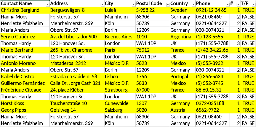
The example below illustrates the preset formatting criteria, such as Duplicate. This formats duplicate contacts with a yellow background.
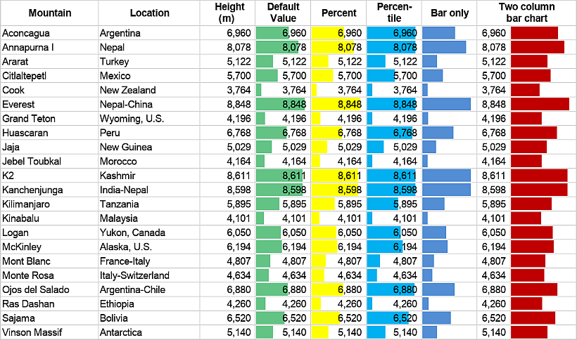
Data Bars Formatting
The Data Bars are used to compare values in the form of a diagram bar.
For example, compare mountain heights by displaying their default value in meters (green bar) and the same value in 0 to 100 percent range (yellow bar); percentile when extreme values slant the data (light blue bar); bars only instead of numbers (blue bar); two-column data analysis to see both numbers and bars (red bar).
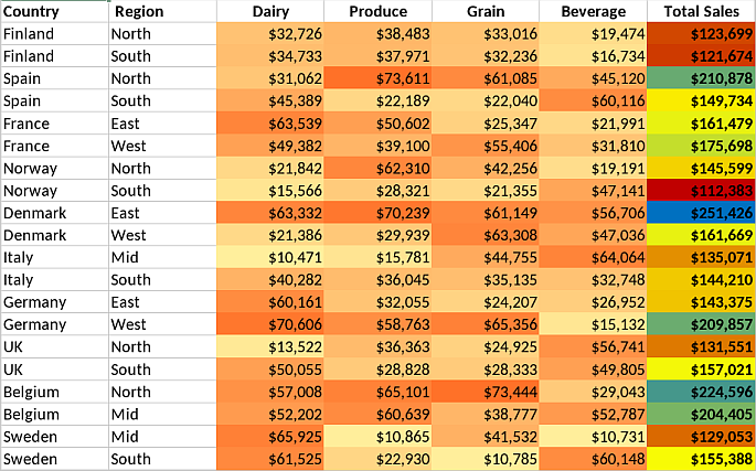
Color Scales Formatting
The Color Scales are used to highlight values within the spreadsheet through a gradient scale.
The example below illustrates the columns from “Dairy” through “Beverage” that display data via a two-color scale with variation from yellow to red; the “Total Sales” column displays data via a three-color scale from the smallest amount in red to the largest amount in blue.
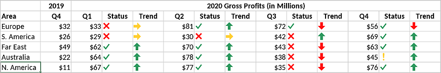
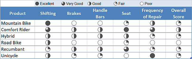
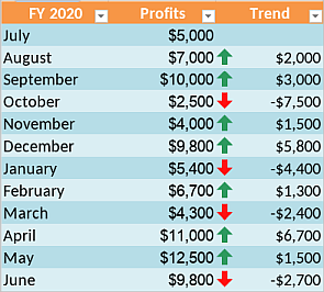
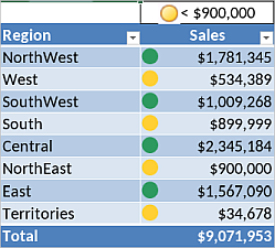
Icon Sets Formatting
The Icon Sets are used to show the data by displaying a corresponding icon in the cell that meets the criteria. The Spreadsheet Editor supports various icon sets:
- Directional
- Shapes
- Indicators
- Ratings
Below you will find examples for the most common icon set conditional formatting cases.
- Instead of numbers and percent values, you see formatted cells with corresponding arrows showing you revenue achievement in the “Status” column and the dynamics for trends in the future in the “Trend” column.
- Instead of cells with rating numbers ranging from 1 to 5, the conditional formatting tool displays corresponding icons from the legend map at the top for each bike in the rating list.
- Instead of manually comparing monthly profit dynamics data, the formatted cells have a corresponding red or green arrow.
- Use the traffic lights system (red, yellow, and green circles) to visualize sales dynamics.
Formatting Using Formulas
The Formula-based formatting uses various formulas to filter data as per specific needs.

- The Rule section shows the selected rule and the selected formatting condition, by clicking the down arrow you can access the list of the available rules and conditions. Use the Select Data box to define the cell value to compare with. Use the reference to a single cell, or the reference with the worksheet function such as =SUM(A1:B5).
- The Format section offers a range of cell formatting options. You can choose one of the available format Presets
or
customize the formatting using font format options (Bold, Italic, Underline, Strikeout), Text color, Fill color and Borders. Use the General drop-down list to choose the appropriate number format (General, Number, Scientific, Accounting, Currency, Date, Time, Percentage). The Preview box shows how the cell will look like after formatting. Click the Clear button to delete all the formatting.
Click OK to confirm.
The examples below illustrate the formula formatting possibilities.
Shade alternate rows,
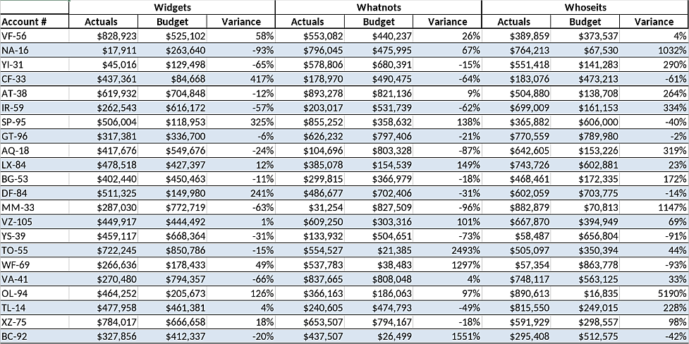
Compare with a reference value (here it is $55), and show if it is higher (green) or lower (red),
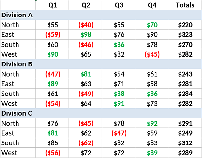
Highlight the rows that meet the needed criteria (see what goals you shall achieve this month, in this case, it is October),
Or, highlight unique rows only
Create New Rule
When you need to create a new rule for conditional formatting, you can do that in one of the following ways:
- Go to the Home tab, click the Conditional Formatting button , and choose New Rule from the drop-down menu.
- Click the Cell Settings tab on the right sidebar and click the Conditional formatting control down arrow, and choose New Rule from the drop-down menu.
- Right-click any cell and choose Conditional Formatting from the contextual menu.
The New Formatting Rule window will open right away. Set the necessary options to configure the rule as described above, and click OK to confirm.
Manage Conditional Formatting Rules
Once you have set up the rules for conditional formatting, you can easily edit, delete and view them using the Manage Rule option by clicking the Conditional Formatting button on the Home tab, or the Conditional formatting control on the right sidebar Cell Settings tab. The Conditional Formatting window appears:
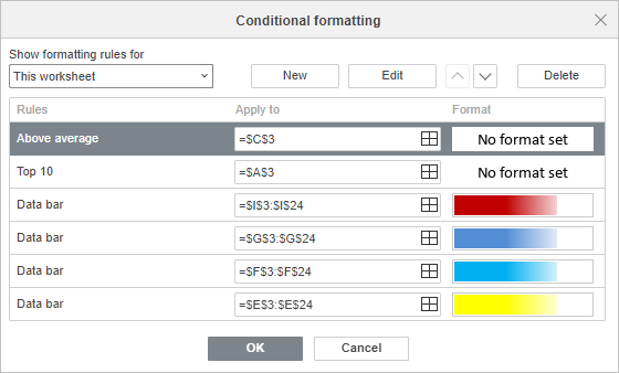
Show formatting rules for allows choosing the rules you wish to display:
- Current selection
- This worksheet
- This table
- This pivot
All rules found in the selected range will be shown in order of precedence (top to bottom) under Rules. The Apply to shows the range the rule is applied to, you can change the range by clicking the Select data icon . The Format shows the formatting rule applied.
- Use the New button to add a new rule.
- Use the Edit button, if you want to edit the existing rule, the Edit Formatting Rule window will open. Edit the rule as you deem it appropriate, and click OK.
- Use up and down arrows to change the place in the order of precedence.
- Click Delete to remove the rule.
- Click OK to confirm.
Edit Conditional Formatting
Editing Value is, Top/Bottom, Average, Text, Date, Blank/Error, Duplicate/Unique, Formula
The Edit Formatting Rule window for Value is, Top/Bottom, Average, Text, Date, Blank/Error, Duplicate/Unique, Formula offers a range of regular settings:

- Click Rule to change the rule and the formatting condition applied previously;
- Use the Select data box to change the cell range to refer to (for Value is, Text and Formula)
- Use the Font and cell format options (Bold, Italic, Underline, Strikeout), Text color, Fill color and Borders.
- Click the General drop-down list to choose the appropriate number format (General, Number, Scientific, Accounting, Currency, Date, Time, Percentage).
- The Preview box shows how the cell will look like after formatting.
- Click OK to confirm.
Editing Data Bars
The Edit Formatting Rule window for Data Bar offers the following options:
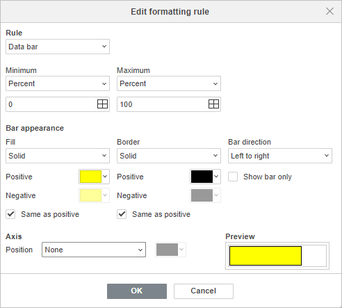
- Rule to change the rule and the formatting condition applied previously;
-
Minimum/Maximum to define the type of the minimum and the maximum values for data bars if you want to focus on differences. The maximum/minimum value types:
- Minimum/Maximum
- Number
- Percent
- Formula
- Percentile
- Automatic
Choose Automatic to set the minimum value to zero, and the maximum value to the largest number in the range. Automatic is the default option.
Click Select data box to change the cell range for the minimum/maximum values.
- Bar Appearance
Customize the Data Bar appearance by choosing the type and the color of the fill and the border, and bar direction.
- There are two Fill type options: Solid fill and Gradient fill. Use the down arrow below to select the fill color for the bars representing Positive and Negative values.
- There are two Border type options: Solid and None. Use the down arrow below to select the border color for the bars representing Positive and Negative values.
- Enable Same as positive check box to display positive and negative using the same color. Color settings for Negative values will be disabled when this box is checked.
- Use Bar Direction to change the direction of data bars. Context is the option by default but you can choose Left to right or Right to left depending on your data representation preferences.
- Enable Show bar only check box to display only data bars in cells and hide values.
- Axis
Select the data bar axis Position in relation to the cell midpoint to separate positive and negative values. There are three axis position options: Automatic, Cell midpoint and None. Click the color box down arrow to set the axis color.
- The Preview box shows how the cell will look like after formatting.
- Click OK to confirm.
Editing Color Scales
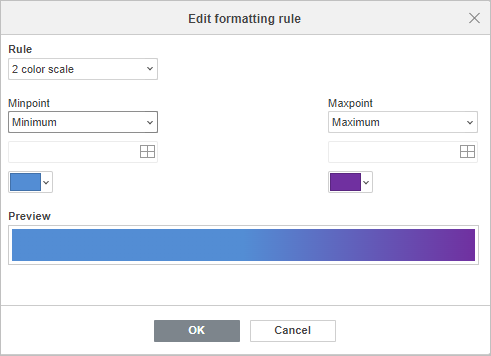
Editing 2 Color Scale Formatting
The Edit Formatting Rule window for 2 Color Scale offers the following formatting options:
Editing 3 Color Scale Formatting
The Edit Formatting Rule window for 3 Color Scale offers the following formatting options:
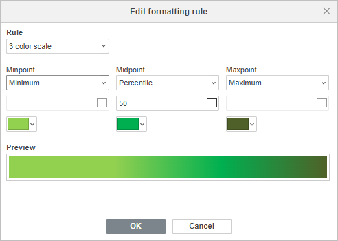
- Click Rule to change the rule and the formatting condition applied previously;
-
Click Minpoint/Midpoint/Maxpoint to define the type of values for the color scale minimum, middle and maximum points if you want to focus on differences.
The minpoint/maxpoint value types:
- Minimum/Maximum
- Number
- Percent
- Formula
- Percentile
The midpoint value types:
- Number
- Percent
- Formula
- Percentile
Minimum/Percentile/Maximum is the default option for 3 Color Scale formatting.
- Use the Select data box to change the cell range for the minimum, the middle and the maximum points.
- Use the down arrow below to select the color for each scale.
- The Preview box shows how the cell will look like after formatting.
- Click OK to confirm.
Editing Icon sets
The Edit Formatting Rule window for Icon Sets offers the following formatting options:
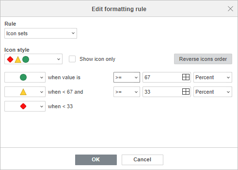
- Click Rule to change the rule and the formatting condition applied previously;
- Click Icon Style to customize the style of the icons for the created rule.
- Enable the Show icon only to display only icons in cells and hide values.
- Enable Reverse Icons Order to change the order of icons and arrange them from the lowest to the highest value. By default the icons are arranged from the highest to the lowest value.
- Set the rule for each icon and adjust comparison operators (greater than or equal to, greater than), threshold values and value type (Number, Percent, Formula, Percentile) to arrange values in sequence from top to bottom. By default, values are divided equally.
- Click OK to confirm.
Clear Conditional Formatting
To clear all conditional formatting go to the Home tab, click the Conditional Formatting button , or click the Conditional Formatting control of the Cell Settings tab on the right sidebar, then click Clear Rules on the drop-down menu, and choose one of the appropriate actions:
- Current selection
- This worksheet
- This table
- This pivot
Please note that this guide contains graphic information from the Microsoft Office Conditional Formatting Samples and guidelines workbook. Try the aforementioned rules display by downloading the workbook and opening it in the Spreadsheet Editor.
Return to previous page